AngioSim

News

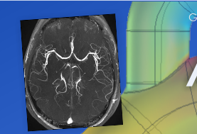
2.12.2015 - Our new paper on simulation of Time-of-Flight and Phase Contrast angiography is now available on-line. We encourage you to read it.

30.11.2015 - In the Downloads section we've added a link to a Xcode project where we implement a vascular tree growth simulation algorithm. Have a try :-).

6.10.2015 - Two new models of the carotid artery bifurcation have been added to the downloads database.

15.08.2015 - We are starting a new project on magnetic resonance simulation. This time we will work on kidney perfusion modeling. More information soon.

Visit also

Visits counter

Number of pageviews from 1/03/2015

Execution acceleration with the use of a computing grid

Simulation of the MR phenomenon involves high computational complexity. The calculation time remarkably increases in case of volumetric acquisitions of high-resolution images. Therefore, one of the project task was to design an efficient multi-processor implementation of the simulator.

The source code was written in the ANSI-C language and compiled for the Mac OS X 10.7 platform (the OS X-native clang compiler was used). Moreover, the program was parallelized using Open MPI library. The algorithm execution is divided into a set of computing agent-nodes, each responsible for handling a given bunch of trajectories. After calculation of the MR signal from its assigned trajectories, an agent sends the results to the master node who adds the received data to the signals simulated by other agents. If there are trajectories still waiting for assignment, an agent who completed its job is employed to handle another portion of data. This procedure ensures high efficiency as more powerful processing resources can be utilized more often. In our experiments the system was installed on the computer grid composed of one iMac desktop (Intel Core i7 3.4 GHz) and 10 MacMini units (10 × Intel Core i5 2.5 GHz) which is equivalent to 24 CPU cores. Additionally, if hyperthreading feature is taken into account, the execution can be distributed among 48 processing slots. The computers were connected over the local ethernet network and communicated on the SSH layer.

The MRA simulation time depends mostly on two factors – the k-space size ($n_x \times n_y \times n_z$) and the number of particles np. The table below presents simulation times measured for different values of these factors and for various grid configurations. The experiments were accomplished for a model of the 50%-stenosis tube.

The measured execution times span from single minutes to approximately 1 h for the most complicated case. These results show efficiency of the system implementation. The duration of a single image synthesis process allows for collecting of their relatively large database in a reasonable time period. It is crucial since large data sample is required for statistically significant evaluation of image processing algorithms.

A comparison of individual measurements reveals that the computational complexity is $O(n_xn_yn_zn_p)$. For example, experiments in rows 1–3 were performed on the same image size but various number of particles $n_p$. As it can be seen, the dependence on the execution time is linear. Similarly, the change on nz (measurements 6 and 7) in relation 1:1.76 (25:44) results in the equivalent increase of the simulation time (in seconds 794:1419). Furthermore, it can be observed (rows 4 and 5) that using hyper-threading technology leads to improved efficiency, although this benefit is lower than the apparent increase in the number of parallel processing slots would suggest.

It must be underlined that the achieved high performance is in part guaranteed by the model itself. Image formation procedures involving the greatest computational burden iterate over particles i.e. actual sources of MR signal but not over every element of the imaged volume (potentially containing the air) as in the other simulators.

Imga size	Number of trajectories	Number of particles	Number of processors	Hyperthreading	Simulation time
128 × 128 × 25	128	71 967	48	Tak	6 m 15 s
		149 386			11 m 24 s
		298 651			23 m 56 s
192 × 192 × 44	256	202 141			53 m 59 s
			24	Nie	1 h 5 m 53 s
128 × 128 × 44			48	Tak	23 m 39 s
128 × 128 × 25					13 m 14 s
			24	Nie	15 m 52 s
			16		22 m 29 s
			10		36 m 25 s

Back