AngioSim

News

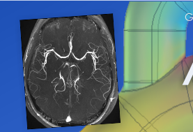
2.12.2015 - Our new paper on simulation of Time-of-Flight and Phase Contrast angiography is now available on-line. We encourage you to read it.

30.11.2015 - In the Downloads section we've added a link to a Xcode project where we implement a vascular tree growth simulation algorithm. Have a try :-).

6.10.2015 - Two new models of the carotid artery bifurcation have been added to the downloads database.

15.08.2015 - We are starting a new project on magnetic resonance simulation. This time we will work on kidney perfusion modeling. More information soon.

Visit also

Visits counter

Number of pageviews from 1/03/2015

Magnetic resonance imaging simulation

The schematic overview of the designed simulator is presented in the figure below. It decomposes into four main function blocks: digital phantom of an organ, sequence management module, simulation kernel, and image reconstruction block.

Schematic of the MRI simulation system.

The digital phantom of an imaged organ

The input to the MRA simulator is a model composed of particle trajectories as described in Flow simulation section. In addition, a phantom may be include components representating stationary tissues which surround vessels. Stationary tissue is modeled by a set of particles similarly to flowing spins but a position of the stationary particle is fixed for the entire scope of simulation. The definition of the stationary tissue requires setting of the shape and size of the organ. Then, the number of stationary particles is adjusted to match the density of their distribution to the ratio obtained for the moving ones. Tissue particles are uniformly distributed within the imaged volume except for the regions occupied by vessel branches. Each particle - both flowing and stationary - is assigned a 3-dimensional magnetization vector, initiated at the beginning of the simulation to the thermal equillibrium state. Next, the state of all magnetization vectors evolves according to imaging sequence events and depending on magnetic parameters of the tissue component they belong to, i.e. proton density ρ, T₁ and T₂ relaxation times. Image formation process is simulated separately for each component. Measurement results are then aggregated before image reconstruction takes place. Optionally, the chemical shift between fat and water components can be defined to simulate spatial misregistration of fat protons caused by magnetic shielding of the electron shell altering their effective resonant frequency.

Distribution of stationary tissue particles around vessels (in blue).

Imaging sequence

The event management module in subsequent simulation steps invokes one of four main procedures which numerically model: 1) RF excitation pulse, 2) free precession, 3) precession under magnetic field gradients, and 4) signal sampling. Theese events sequence is repeated in accordance with timing configuration: TR - repetiion time (interval between subsequent RF pulses), and TE - echo time (interval between RF pulse application and half time of the signal acquisition window). In the MR imaging, there exist two main measurement sequences - spin echo (SE) and gradient echo (GE). Both sequence types are implemented in the designed simulator. However, in the angiography domain, only the GE sequence is employed. Additional parameter for the GE sequence is the flip angle (FA) of the magnetization vector relative to the direction of main magnetic field B0. FA determines the level of spins excitation, i.e. the lenght of their magnetization vectors projection onto the transverse plane. The sequence management module also embraces the complete definition of the measurement protocol, including the scanning options, such as

flow compensation,
ramped flip angle (TONE),
Multiple Overlapped Thin Slab Acquisition (MOTSA).

Signal computation

The designed MR simulation module uses the analytical approach to solving the Bloch equation. Thus, in the matrix-based formulation the longitudinal and transverse relaxation processes of the magnetization vector $\mathrm{\textbf{M}}$ of a particle $p$ during the time interval $\delta t$ are given by
$$\mathrm{\textbf{M}}_p(t + \delta t) = Rot_z(\theta_g)Rot_z(\theta_i)R_{\mathrm{relax}}^{12}\mathrm{\textbf{M}}_p(t) + R_{\mathrm{relax}}^{1}\mathrm{\textbf{M}}_0,$$ where $Rot_z$ determines the rotation of $\mathrm{\textbf{M}}_p$ around the $z$ axis due to the phase encoding gradient ($\theta_g$) and field inhomogeneity effect ($\theta_i$). $R_{\mathrm{relax}}^{12}$ and $R_{\mathrm{relax}}^{1}$ account for the transverse and longitudinal relaxation phenomena:
$$R_{\mathrm{relax}}^{12}=\left( \begin{array}{ccc} e^{-\frac{\delta t}{T_2}} & 0 & 0\\ 0 & e^{-\frac{\delta t}{T_2}} & 0\\ 0 & 0 & e^{-\frac{\delta t}{T_1}} \end{array} \right),$$ $$ R_{\mathrm{relax}}^1=\left( \begin{array}{c} 0\\ 0\\ 1 - e^{-\frac{\delta t}{T_1}} \end{array} \right). $$ The equilibrium magnetization $\mathrm{\textbf{M}}_0$ depends on several factors, including Planck and Boltzmann constants, gyromagnetic ratio, as well as tissue temperature and proton density. In the current system implementation $\mathrm{\textbf{M}}_0$ is determined exclusively in relation to proton density, which ultimately only scales the signal magnitude but does not affect spins net behavior.

Note, that for the proper evaluation of the Bloch equation, position of a flowing particle relative to gradient isocenter must be determined first. Thus, a magnetization vector has to be updated at time intervals which ensure reasonable trade-off between precision of the flow simulation, MR modeling and computational burden. Too high values of $\delta t$ introduce unacceptable discontinuity in evolution of the effective Larmor frequency experienced by a particle. On the other hand, very short $\delta t$ results in significant increase in simulation time. In our approach, $\delta t$ is set to match signal sampling interval. However, $\delta t$ is a fully independent parameter of the simulator and can be adjusted for specific application to any desired value.

Since the assumed duration of the excitation pulse is much shorter than relaxation times, the post-pulse magnetization is calculated from
$$ \mathrm{\textbf{M}}_p(t + \delta t) = R_{\mathrm{RF}}\left(\alpha_{\mathrm{eff}}\right)\mathrm{\textbf{M}}_p(t). $$ $R_{\mathrm{RF}}$ flips $\mathrm{\textbf{M}}_p$towards transverse plane by an effective angle ($\alpha_{\mathrm{eff}}$). This term encapsulates off-resonance conditions which changes the assumed flip angle $\alpha$. Finally, signal acquisition is accomplished by summing up contributions from every particle $p$ in the k-space: $$s(t) = \sum_{p=1}^{n_p}\vec M_p(t)\vec x + j\sum_{p=1}^{n_p}\vec M_p(t)\vec y,$$ where $n_p$ denotes the total number of particles in the vessel. Readout window is divided into $n_x$ steps – the size of k-space in the frequency encoding direction. Between the sampling steps blood particles move and their magnetization vectors evolve. At the end of the readout window one line of k-space is filled in.

Image reconstruction

The last stage of image formation procedure consists in transformation of the raw data in the spatial- frequency domain (K-space) into image intensity domain. This stage is accomplished by the fast Fourier transform, followed by calculation of the magnitude of – complex transformation output. Before application of the FFT routine, it may be necessary to filter the raw data to reduce the phase mismapping artifact appearing in the phase encoding direction due to the motion of blood particles. We decided to port the filtering routine and FFT-based image reconstruction to the Matlab environment to enable any kind of low-pass digital filter available in the Signal Processing Toolbox to be used.

Back