


| About | Downloads | Publications | Contributors | Achievements |
| News |
|
2.12.2015 - Our new paper on simulation of Time-of-Flight and Phase Contrast angiography is now available on-line. We encourage you to read it.
30.11.2015 - In the Downloads section we've added a link to a Xcode project where we implement a vascular tree growth simulation algorithm. Have a try :-). 6.10.2015 - Two new models of the carotid artery bifurcation have been added to the downloads database. 15.08.2015 - We are starting a new project on magnetic resonance simulation. This time we will work on kidney perfusion modeling. More information soon. |
| Visit also |


|
| Visits counter |
|
Number of pageviews from 1/03/2015 |
Flow simulation
Blood flow
A simulation of flow is performed in COMSOL Multiphysics software. The routines implemented therein solve Navier-Stokes equations for the incompressible fluid. A laminar flow, known also as stratified flow, assumes that fluid moves in parallel layers. Each layer has its own speed and slides past one another with no lateral mixing. Blood flows in one direction with the parabolic velocity profile reaching the greatest value in the middle of the cylinder and it decreases towards vessel walls. The model is sufficiently accurate for simulating blood flow in a straight tube of relatively large diameter. However, in case of more complex structures with stenoses and bifurcations the flow behavior locally changes and turbulences and frictional forces should be taken into consideration. Therefore, in the presented study the flow simulation is conducted in the turbulent regime using the RANS k-ε equation.
Among other available options, fluid motion in a vessel can be forced by determining pressure difference between the inlet and outlet surfaces. From the physiological point of view, the reasonable rates of peak velocity of blood for medium and large arteries (such as those modeled by the Shelley phantoms) range from 30 to 100 cm/s and the pressure values must be adjusted accordingly. In the example presented below a simulated distribution of pressure and velocity inside digitally reconstructed phantoms, where input and output pressure values were set to 11168 Pa and 11148 Pa respectively. In this case, the maximum magnitude velocity of the flowing blood amounts to 8 cm/s.
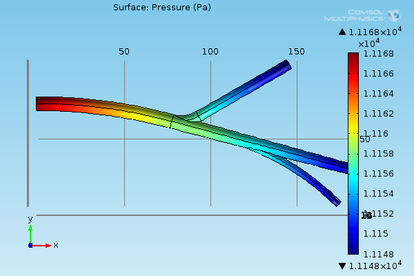
Pressure distribution on the vessel walls determined based on blood flow simulation.
Transport of magnetization
t is important to note that COMSOL splits the domain of interest (in our case – the fluid) into a mesh of 3D geometrical primitives – tetrahedral nodes – of some finite volume. Velocity vectors are calculated for every mesh node. A crucial issue, is how to transfer this information in a usable form into the virtual MR scanner. A direct approach involves an operation on the COMSOL-generated mesh but it breeds a problem, referred to as numerical diffusion. An example of fluid motion in the next figure, showing positions of a portion of blood in 3 subsequent time steps, illustrates the problem.
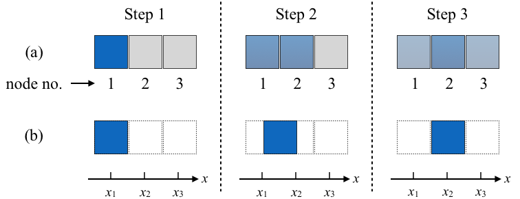
Illustration of numerical diffusion problem.
If the flow channel is decomposed into a mesh of regular square-shaped nodes (in fact, any shape of mesh primitives entails similar consequences) it seems that in step 2, only half of the fluid volume shifts from node 1 to node 2. Thus, any further mesh-based calculations would require a division of fluid volume of this particular blood portion into 2 fractions, each for nodes 1 and 2. In step 3, these fractions move on: a part of blood residing in node 2 is transported to node 3, and again only a fraction of node 1 volume shifts towards node 2. Apparently, a sample of blood which initially occupied only one mesh node, spilled over 3 nodes. Clearly, this leads to an ambiguous localization of fluid portions – an error which accumulates in subsequent time steps. Moreover, this problem affects simulation of magnetic resonance, where subsequent image formation procedures (selective excitation, spatial encoding etc.) are invoked in discrete time moments and applied to portions of fluids at specific locations. Hence, a numerical diffusion may cause misinterpretation of true position of some blood samples.
Particle trajectories
To avoid the above described problem another COMSOL toolbox, namely the Particle Tracing for Fluid Flow module is used. Based on the laminar and turbulent flow solution, the group of particles fed into a tube at an inlet is transported to its outlet. Each spherically-shaped particle is described by its density and diameter. Furthermore, the simulation is configured in such a manner, that there is no particle-fluid interaction. On the other hand, fluid forces particles to move along a vessel and by tracing their locations in subsequent time steps it is possible to find a bundle of trajectories which represent the motion of blood. These particle trajectories define the input to the MRA simulator. Below, particle trajectories obtained for the above-presented flow simulation result are shown.
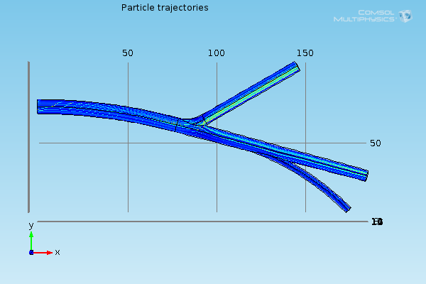
Example particle trajectories.
These trajectories are then populated with particles (or moving spins) on their entire length, so that the whole volume of a vessel tree is filled with them. The particles are spaced in such a way, that the distances between them are basically proportional to the local velocity at a given streamline. As the local velocity increases, e.g. at a narrowing, the distances between particles is also enlarged, so that the assumption of fluid incompressibility is sustained. This step is accomplished by a separate module, which keeps track of positions of all individual particles identified by their trajectory number and a unique label. As the simulation progresses, new particles flow into a vessel tree replacing those which flow out. The routine is capable of determining spin locations with arbitrary temporal resolution. Watch the on-line video manual which illustrates the operation of the described module.